I recently was asked to generate an emailed reminder for actions following meetings. This solution was put into place to do this, but rather than send out an email reminder per action, this combines all outstanding actions for each user and sends them a single email, with a link to update each item.
The end result looks something like this:
This was done in part by using a useful formula in Google I had been unaware of until recently, "REPT" Combined with CONCATENATE, this can pull through matching items from another range of cells.
e.g. in my demo sheet the formula =ArrayFormula(concatenate(rept(Outstanding!L:L&" ",Outstanding!C:C=A3)))
brings in all items from column L in one sheet, where Column C in that sheet matches cell A3.
In the demo sheet, this formula brings through some concatenated HTML table code which wraps the data for each line.
Progress stars correspond to a Google form Linear Scale question (1 to 5) with a simple formula to select the appropriate image.
So that only those with actions get sent emails, I used a query to just bring in items with less than 5 stars (complete) and then a pivot query on those items.
For the scripts - I just set up the getEditResponseUrls script to run on Form submit (change the Form URL in the script to yours before doing this) and the sendweeklyemail script to run on a timer.
Another tweak that would need to be made would be to amend the form to put in the list of names for the actions, replacing the ones in there, and putting in the matching names and email addresses in the Vlookup tab in the Google Sheet.
The demo sheet is also set up to display easily in an Awesome Table as per the example below
Hope this is of interest, any questions please let me know
Google recently added an attachment upload function to Google GSuite customers. This functionality has replaced some workarounds, including one I have blooged about before using Folders
Google creates a Drive folder for the attachments, and lists the attachments URLs in the response sheet, separated by commas. This is great, but to display the information in a Google site or similar, it is most useful to use an Awesome Table to display the results. To get this formatted to suit an Awesome Table is a bit fiddly however. This post explains a way to get this set up
To begin with I created a new tab which is the one that the Awesome table will read from, manually inputted the column names in the first row, added filters on the second, and in the third row added in a query to bring the data in from the form.
As the file URLs are all in one column, separated by a comma and a space, it would not be possible to hyperlink these with a formula - the files need to be split out initially - this is done with an array formula with a split function, using ", " as the separator
Next a Google Apps script was added to list the URLs and names of the folder that was created automatically to contain the form attachments. The code should be set on a trigger, on form submit.
The script formats the URL to match the same syntax that the Google form produces and will output to a tab I created called 'FileList'.
function search()  {

    var folder =  DriveApp.getFolderById("***INSERT YOUR GOOGLE DRIVE FOLDER ID HERE**");

  var files = folder.getFiles();


     var sheetName = 'FileList';

var SheetIds = 2;

var sheet = SpreadsheetApp.getActiveSpreadsheet().getSheetByName(sheetName);

  sheet.clear();

  sheet.appendRow(["URL","FileName"]);

 while (files.hasNext()) {

   var string = 'https://drive.google.com/open?id=';
   var file = files.next();
   Logger.log(file);
   Logger.log(string);
 var data;
    data = [
      string + file.getId(),
     file.getName(),


    ];

    sheet.appendRow(data);

  }
  SpreadsheetApp.flush();


};
End Result is as per the below screenshot when it runs
Now we have the URL and the Name, vlookups can be added to each of the 'Doc' columns to bring through the filenames
With all this done, the final step is to add a tab called template, which can then be used in the Awesome table setup. Screenshot below, but the file is linked at the end of this post, in case you want to copy and paste. The documents column takes the URLs and file names and hyperlinks each one with a generic document icon
In the Awesome Table setup - just reference the template to apply this
We recently had a requirement for users to complete a short assessment, to record which users passed, and for those who did, to receive a certificate.
To do this I used Google Apps script, Google Apps and a great add-on, Form Publisher
Here's a diagram of how it all works...
In the background collection sheet of the assessment quiz, formulae work out whether the answers are correct and score them a 1 or a 0 - A formula at the end assigns either a 1 (pass) or a 0 (fail) based on the target score. Those who have achieved a pass mark, have their details pulled through into another tab, using a simple query. e.g =query('Form responses 1'!Y2:AE,"select Z,AA WHERE (Y=1)")
A similar tab can be created to pull through those who have failed just using Where =0 instead
How to then pass the details into a certificate is achieved using Google Apps Script. This script populates a new form, which uses the Form Publisher add-on and submits it.
var sheetName = 'Mail Merge'; // enter the name of the sheet

function GenerateCertificate() {

  var CERTIFICATE_CREATED = "CERTIFICATE_CREATED";  //Define flag used to stop duplicates

  var form = FormApp.openById('abcdefghijklmnopq123456789');  //your form id goes here
  var sheet = SpreadsheetApp.getActiveSpreadsheet().getSheetByName(sheetName);
  var rows = sheet.getDataRange();
  var numRows = rows.getNumRows();
  var values = rows.getValues();

   var data = sheet.getDataRange()  // Get all non-blank cells
   .getValues()     // Get array of values

      var startRow =1;  // First row of data to process

   for (var i=0; i<data.length; i++){

    var formResponse = form.createResponse();
    var items = form.getItems();

    var row = data[i];
         var processedstatus = row[4];  // column - Column containing the flag to stop duplciates  (A=0)

      if (processedstatus != CERTIFICATE_CREATED) {     //If Flag text not found then.....

        //Take the first column data and input this into the next form  (e.g Full Name)
     var items = form.getItems(FormApp.ItemType.TEXT)
     var formItem = items[0].asTextItem();
    var response = formItem.createResponse(row[0]);
    formResponse.withItemResponse(response);

         //Take the second column data and input this into the next form (e.g. Name of assessment)
    var formItem2 = items[1].asTextItem();
    var response = formItem2.createResponse(row[1]);
    formResponse.withItemResponse(response);

        //Take the third column data and input this into the next form  (e.g. date completed)
    var formItem3 = items[2].asTextItem();
    var response = formItem3.createResponse(row[2]);
    formResponse.withItemResponse(response);

        //submit the form
    formResponse.submit();
    Utilities.sleep(500);

        //set the flag to stop duplicates
      sheet.getRange(startRow + i, 5).setValue(CERTIFICATE_CREATED);

       SpreadsheetApp.flush();
      }

  }

};
The script will only process those rows without the flag "CERTIFICATE_CREATED" in column E, once it has processed that row, it adds that text, to prevent duplicates being created.
In the background, when the script populates the user name, assessment and date into the next form and submits it. Form Publisher merges the fields into a certificate template I set up in Google Slides, saves the certificate as a pdf, and then emails it to the person who took the test.
A useful feature of using a second form, processed by a script, is that sheets for different assessments / courses can use that same template and same 'certificate generator' form to create appropriate certificates. All that is needed is the script in a background collector sheet to populate that form with the required data.
{NB A copy of the sheet with all the formula used in this demo can be found here]
The National Institute of Health Research (NIHR) publish an annual table of national research activity. In this demo, I am going to use this dataset in Google sheets, by extracting a subset of the information from the website with a formula, and then using a few different pivot formula to manipulate the data.
To extract just the information for NHS organisations in Kent, Surrey and Sussex, in my Google sheet I have used the formula
=query(importhtml("http://www.nihr.ac.uk/research-and-impact/nhs-research-performance/league-tables/league-table-data.htm","table",1),"SELECT Col1, Col2, Col3,Col4,Col5,Col6,Col7,Col8 where Col3 ='Kent, Surrey and Sussex'")
Simple pivot
To pivot the results, you can use a pivot table in Google sheets, via the data menu, However you can also use a formula to generate a pivot
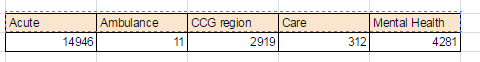
Here's a simple example (where the raw data is on a sheet called "Raw Data 1" - showing the number of recruits by organisation type.
=query('Raw Data 1'!A:H, "select sum(H) pivot B")
Transpose a pivot
To change the orientation, so that it looks more like a normal pivot table, you can use 'transpose' in the formula
=transpose(query('Raw Data 1'!A:H, "select sum(H) pivot B"))
Filter a pivot
You can also apply a filter parameter in your query, so for example the following shows the sum of recruitment for just Acute trusts
=transpose(query('Raw Data 1'!A:H, "select sum(H) where B ='Acute' pivot A "))
Use multiple columns in a pivot
You can also bring other columns into a pivot, as long as these are included in the 'group by' or wrapped in an aggregate function. I have used a 'where' clause too to prevent blank rows being included in the pivot
=query('Raw Data 1'!A:H, "select A,sum(H) where G >0 group by A pivot B")
Sorting a pivot
Sorting a pivot is more tricky, in the example below, I have used a query, to query the query ;-)
=QUERY( TRANSPOSE((query('Raw Data 1'!A:H, "select sum(H) where B ='Acute' pivot A"))) , "Select Col1,Col2 Order by Col2 desc ")
****Update August 2017 - Due to recent changes by Awesome Table to their background code, this solution no longer will work. Ill try to revisit this in future to see if a revision to the code below can get this working again, time permitting*****
This solution came about from a requirement we had for colleagues to easily add updates and comments to a monthly report which was itself refreshed each month with new data. As the data changed in the report it was necessary to find a way to get the existing comments to be kept and to show against the appropriate matching lines in the new data set. To do this, I used an Awesome Table, with a sidebar, linked to a form which could be toggled to show and hide. The form has a few fields which are pre-filled depending on the line of data, so that the comments then get matched up and shown in the table.
A demo of the solution is below, using some dummy data (a copy of the spreadsheet can be found at the bottom of the post)
To start I created a Google Sheet with the data in and a Google form to collect the comments
To get a unique value per row that can match against the appropriate comment, I concatenated the first three columns of my data (Trust, site and study ID). The formula puts the title of the column in the first cell, 'Nofilter' in the second cell (used to define the Awesome Table filter) and in the remaining rows with data, the concatenation:
=ArrayFormula(IF(ROW(A:A)=1,"Concatenate",IF(ROW(A:A)=2,"NoFilter",IF(LEN(D1:D),(D1:D&"|"&C1:C&"|"&B1:B),IFERROR(1/0)))))
with a similar formula on the form result sheet, any matching results can be brought in with a query, but with a join function, to combine multiple matching entries, sorting the matching comments by most recent.
=join("",query(Comments!A$2:H,"select G Where A = """&A3&""" order by B desc"))
(NB - one annoyance is that the query cannot be combined with an array formula, so this formula is filled down in a standard way. If the data is submitted via a form as well, then an Importrange or a query function can always be used to bring in that data to another sheet which would then be used for the remaining calcs.)
The returned column combines the date stamp, formatted to show just the date, with the comment, and some HTML line breaks so that this displays well in the Awesome Table, which was obtained by the following formula.
=ArrayFormula(TEXT(B2:B," dd/mm/yy - ")&F2:F&"<br/><br/>")
Awesome Tables now use Templates which is a fantastic new feature. In the template I added
what would appear in the sidebar, which is an iframe of the form, prefilling three of the fields using the data in the rows.
I then added some JavaScript to the template so that when a button is clicked, the sidebar is shown or hidden, with the table width expanded or reduced accordingly.
Update March 2017 - A file upload feature has now been added to Google forms for GSuite customers for forms within their domain. To get an Awesome Table to work with this new feature, see my blogpost here Update December 2015 - for enhancements such as automatically sharing folders with recipients and a link directly to the folder view rather than the 'open in drive' view, please see responses to comments below this post
Google forms are really useful, but a limitation is that it is not possible to attach a document to a record (as you can do with a SharePoint list for example)
This script aims to give a workaround for that - when a user submits a form, the form entry is assigned a unique reference, a Drive folder is created with that reference, and they receive an email containing a link to that folder to upload related documentation. Using an Awesome table, the link to the folder as well as the details in the form can be displayed together to make it easy to match documents to form items.
To being with, I created a Google form, and a Google sheet to collect the information.
To create a unique reference I used the following formula in the first row of the first empty column (where a username is in column B) The formula puts the title "Reference" in the first row, in the second row it puts "NoFilter" (for use in the Awesome Table) and for any subsequent lines, it takes the first letter of the users first name, two letters from the surname, and the row number to make the unique reference
var formURL = 'https://docs.google.com/a/nihr.ac.uk/forms/d/0123456789abcdsefghijklmnop/edit'; // enter the edit url for the form
var sheetName = 'Form responses 1'; // enter the name of the sheet
var columnIndex = 8;  //the number here is a count with A = 1, it indicates where the link should go

// script to get the edit link

function getEditResponseUrls(){
  var sheet = SpreadsheetApp.getActiveSpreadsheet().getSheetByName(sheetName);
  var data = sheet.getDataRange().getValues();
  var form = FormApp.openByUrl(formURL);
  for(var i = 2; i < data.length; i++) {
    if(data[i][0] != '' && (data[i][columnIndex-1] == '' || !data[i][columnIndex-1])) {
      var timestamp = data[i][0];
      var formSubmitted = form.getResponses(timestamp);
      if(formSubmitted.length < 1) continue;
      var editResponseUrl = formSubmitted[0].getEditResponseUrl();
      sheet.getRange(i+1, columnIndex).setValue(editResponseUrl);
    }
  }
}

// script to create a folder for document uploads

function createFolder () {

var FOLDER_CREATED = "FOLDER_CREATED";

  // Get current spreadsheet
  var ss = SpreadsheetApp.getActiveSpreadsheet();
  var sheet = ss.getSheetByName("Form responses 1");
  var data = ss.getDataRange()  // Get all non-blank cells
               .getValues()     // Get array of values
               .splice(2);      // Remove header lines

  // Define column number unique reference. Array starts at 0.
  var CLASS = 6;  //column G

// Get the ID of the root folder, where the sub folders will be created
  var DriveFolder = DriveApp.getFolderById("0123456789101112131415161718abcdefghijklmnop");

  // For each email address (row in a spreadsheet), create a folder,
  // name it with the data from the Class

  for (var i=0; i<data.length; i++){

    var startRow = 3;  // First row of data to process
    var row = data[i];
    var class = data[i][CLASS];
    var folderName = class;
    var supplier = row[3];  //column D
    var folderstatus = row[9];  // column J

   if (folderstatus != FOLDER_CREATED) {

  //create the folder
  var folderpath = DriveFolder.createFolder(folderName).getUrl();

//send an email

  var emailAddress = row[2];  // Column C)
  var message = 'Thank you for submitting a purchase order requisition for supplier: '+ supplier +' - please upload the purchase order(s) relating to this to the following folder ' +folderpath ;

      var subject = "Please upload related documentation";
     MailApp.sendEmail(emailAddress, subject, message, {
  //  cc: 'sample@email.com'         // optional cc

 });

      //set the flag to avoid duplicates
      sheet.getRange(startRow + i, 10).setValue(FOLDER_CREATED);
      sheet.getRange(startRow + i, 11).setValue(folderpath);
      // Make sure the cell is updated right away
     SpreadsheetApp.flush();

         }

    }
  }
Both scripts should be set to trigger when the form submits.
When a user enters information in the form, the scripts will generate an edit link to the item, and create a Drive sub folder with the unqiue ID. They then will get an email which contains a link to the newly created folder...
On a Google site, the results can be displayed in an Awesome Table...
The Awesome Table setup used is below:
One quick note, as the unique ID is generated from the row number, deleting a row in the sheet would cause a mismatch between the references and any already created folders...
In my example above in the 'Advanced parameters', the Awesome Table is set to only show rows where A is not blank, so the method for removing any unwanted records from displaying in the Awesome table should just be a matter of deleting the timestamp for the unwanted row in the sheet.
Hope this is of interest. A copy of the demo sheet, including scripts can be found here
Google forms have some great strengths, particularly in the way that Google Apps Scripts can work with the collected data. There's not much you can do though to the out of the box Google form to add functionality such as comparing fields for validation, adding word counts or any other JavaScript tricks. A way of getting the best of both worlds is to extract the Google form and put it into a web page, which can be hosted on Google Drive, and then enhance the design and functionality as you like with HTML and JavaScript.
The below video shows a few of the enhancements - including
-automatic word counts as you type in paragraph text fields
-email address and tickbox validation to prevent form being submitted unless boxes are ticked
-accordion dropdowns to reduce form size
-working hyperlinks in the text.
While these features are in the front end, in the back, as the fields are all still Google form fields, there is functionality in the collecting Google sheet so that when the form is submitted, Google Apps Scripts run, to provide an edit link, emailing the recipient with confirmation of the data and a link to edit, and a set timer so that the recipient is contacted every x months to review their data and amend if necessary. As normal with Google sheets, an add-on can alert the owners of the sheet when a form is submitted, and Awesome tables can summarise the data and provide searching and filtering.
Some of the code snippets are below:
I included a reference to jquery in the <head> for the accordion and field validation scripts
If you have fields set to required in the Google form, if you try to submit the webpage version without completing these fields, then you are taken to the original Google form to complete these. This clearly isn't ideal, so its necessary to make the fields required instead using JavaScript
Sample code here for one of the fields
<script type="text/javascript">
// validate the First Name field
$('form').submit(function () {
    // Get the Login Name value and trim it
    var name2 = $.trim($('#entry_12345678').val());
    // Check if empty of not
    if (name2  === '') {
    $('#errorwarning2').text("Required field 'First Name' is empty, please correct and re-submit.");
        return false;
    }
});
</script>
To do a word count, I used the following script
<script type="text/javascript">
function wordCount( val ){
    return {
        charactersNoSpaces : val.replace(/\s+/g, '').length,
        characters         : val.length,
        words              : val.match(/\S+/g).length,
        lines              : val.split(/\r*\n/).length
    };
}
var $div1 = $('#count1');

$('#entry_987654321').on('input', function(){
var a = wordCount( this.value );
$div1.html(
"<br>Word count: "+ a.words
);
});
</script>
The Div that shows the word count can then be put next to the relevant field
To stop the form submitting if the email address fields do not match, I used the following:
<script type="text/javascript">

// form id value, default is ss-form
var formID = 'ss-form';
var formKey = 'abcdefghijklmnop123456789';
var submitted = false;

$(document).ready(function () {
    var ssForm = $('#' + formID);

    ssForm.submit(function (evt) {
         var email = document.getElementById("entry_123456789").value;
        var confemail = document.getElementById("entry_1011121314").value;
if(email == confemail) {
            ssForm.attr({'action' : 'https://docs.google.com/forms/d/' + formKey + '/formResponse'});
            return true;
        } else {

    $('#errorwarning').text("Error - email addresses do not match, please correct and re-submit.")
            return false;
        }
    });
});
</script>
If the user has mistyped an email address and has been unable to submit the form, I wanted the error message relating to this to hide as soon as they start typing in the email field again. For this I just used this: